This tutorial will teach you how to do K-Means Clustering in SAS. It also explains the various statistical techniques used in cluster analysis with examples.
Cluster analysis is a type of multivariate data mining that groups items (like products, respondents, or other entities) based on characteristics or attributes chosen by the user.
It is the first and most crucial step in data mining. It is a common way to look at statistical data and is used in many different areas, such as data compression, machine learning, pattern recognition, and finding information.
What is cluster analysis?
Let’s first understand how K-Means clustering works. K-means clustering is an algorithm for machine learning that puts together small groups of similar data points that haven’t been labelled.
For example,
We have a large number of students belonging to a particular university. Since this is an unsupervised algorithm, the students are not put into groups or classes.
Think of this as a picture of all the students in a space with many dimensions.
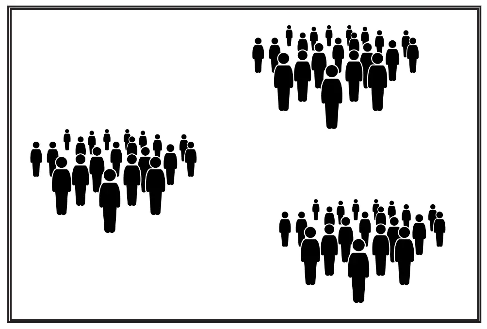
After implementing the K Means clustering algorithm, we obtain the following clusters:
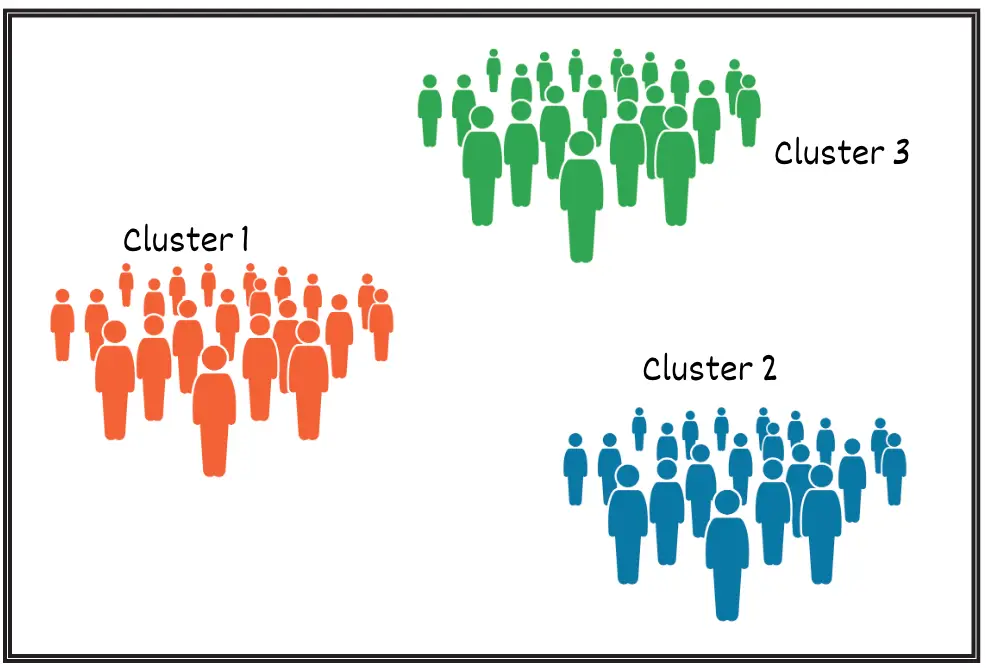
On further inspection, we found that-
- Students belonging to Cluster 1 are computer science students.
- Students belonging to Cluster 2 are Medical students.
- Students belonging to Cluster 3 are Economics students.
K Means clustering helped us to logically separate them into three groups.
These groups are called clusters when we try to group a set of objects with similar characteristics and attributes. The process is called clustering.
Data points in one cluster are entirely different from those in another. However, all the data points in the same cluster are either the same or related.
Steps in Clustering
Before proceeding, let us know the definition of a centroid
The centroid point is the point that represents its cluster. The centroid point is the average of all the points in the set and will change its value when a new data point gets added in each step. It is computed using the below formula:
For the above equation,
C_i: is the i’th Centroid
S_i: it is all points belonging to cluster_i with centroid as C_i
x_j: j’th point from the set
||S_i||: number of points in cluster_i
Now, let us know about the internal procedures of K Means clustering.
Let’s say we have a Dataset with two variables, x and y.

Step 1: Defining the number of clusters: K-means clustering is a type of non-hierarchical clustering where K stands for K number of clusters.
As a first step, we must determine the value of K. When K=3, the algorithm will divide the data points into three clusters based on their characteristics. Accordingly, if we give K=5, the algorithm will group the data points into 5 clusters based on their features.
So, to get some logically acceptable groups, we need to find the optimal value of K. Various methods can be used to do this, such as the elbow method, trial and error, etc.
For more details o methods for choosing the right number of clusters, refer to this article.
However, we won’t dwell on that too much. Instead, let’s suppose that we obtained the value of K as 3 after implementing the elbow method.
Step 2: Define the Centroid of each cluster: K-means clustering is an iterative procedure to define the clusters. This step is the starting point at the centre of each cluster.
Initialize the ‘K’ number of centroids randomly in the multidimensional space (Here, K=3). The initial centroid is placed in random locations in the first iteration.
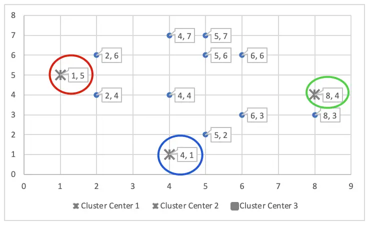
The initial cluster centres – means are (1, 5), (4, 1) and (8, 4) – chosen randomly. They are also called cluster seeds.

Step 3: Calculate the distance of each data point to the centre of each cluster one by one. Assign the data point to that cluster that has the smallest Euclidean distance.
The distance can be measured in many ways. Two of the most popular methods are as follows:
Euclidean distance =
Manhattan distance =
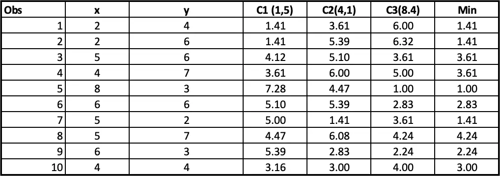
Step 4: Allocating clusters to all the observations: The next step is to allocate clusters to each observation. We will do that by using the min(cluster 1 value, cluster 2 value) from step 3. So for the first obs, the minimum value for cluster 1 (2 vs 4) is 1.41. so observation 1 belongs to cluster 1. The minimum value for the second obs is for cluster 2 (2 vs 6), so the second obs belongs to cluster 1, and so on.
We must follow the same steps to optimize cluster allocation using different centre points. This can be done through different iterations.
Step 4 should be repeated until the centroids’ positions do not change.
Iteration 1:

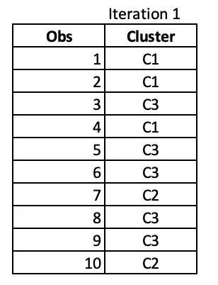
At the end of 1st iteration, we have the cluster assignments as follows.
Iteration 2:
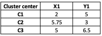
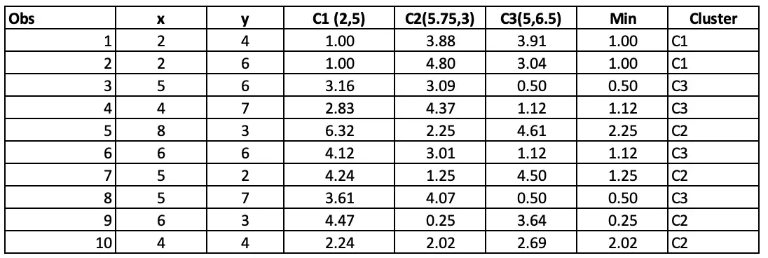
Until now, we did only iteration 1, picking centre points randomly. Now, we will pick the centre points based on iteration 1 output as follow:
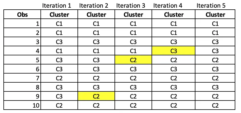
Observations 1, 2 and 4 belong to cluster 1, and the rest belongs to cluster 2 and Cluster 3, respectively. So, we will take the average of all the points grouped by cluster to set the new centre points in iteration 2.


If we update the centre points in iteration 2, the distance will also change, and hence, the final cluster will also change as follow:
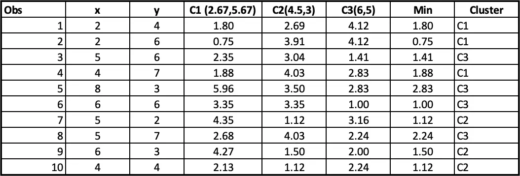
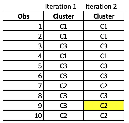
Notice that observation 9 has moved from cluster C3 to C2 after iteration 2.
Iteration 3:
We again take the average and update the centre points in iteration 3. Again the distance and final cluster will get changed as follow:

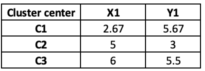
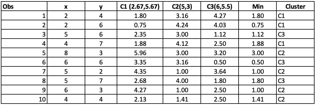
In Iteration 3, Observation 5 has moved from C3 to C2.
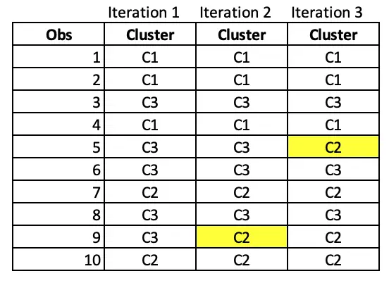
Iteration 4:

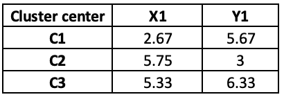
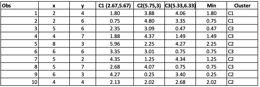
At iteration 4, Observation 4 has moved from C1 to C3.
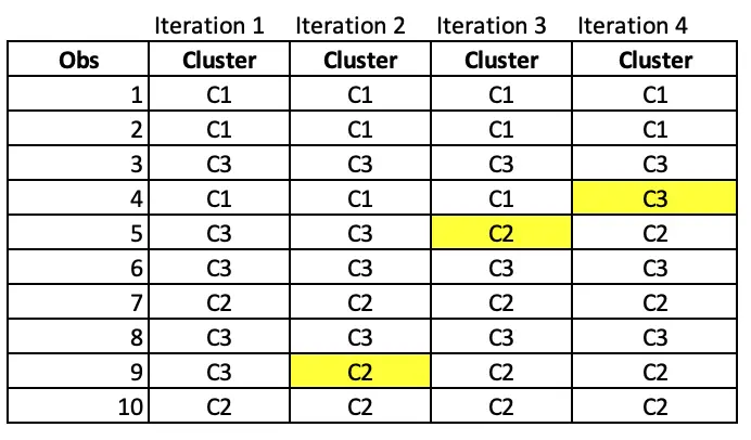
Iteration 5:

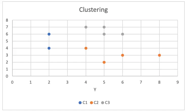
As cluster allocations are not changing even if we perform iteration 5, we can now say that the algorithm is converged. We now have an optimum cluster allocation(that is, cluster from iteration 5).
Cluster Analysis in SAS
Let’s take the famous IRIS datasets.
Each flower in this dataset is categorized as Setosa, Versicolor or Virginia and measurements SepalLength, Sepalwidh, PetalLength and Petalwidth.
Checking the dataset by using proc means.
proc means data=sashelp.iris N Nmiss mean median max min stdev;
run;
It has 150 observations and 5 variables. No missing values or outliers were detected. We will use only four variables, namely sepal_length, sepal_width, petal_length and petal_width.
Before running cluster analysis, we need to standardize all the analysis variables (real numeric variables) to a mean of zero and a standard deviation of one (converted to z-scores).
proc stdize data=SASHELP.IRIS out=iris_std_ method=range;
	var Sepallength Sepalwidth petallength petalwidth;
run;
The STDIZE procedure is first used to standardize all the analytical variables to a mean of 0 and a standard
deviation of 1. The procedure creates the output data set Stand to contain the transformed variables (for
detailed information, see our post on the Standardization of variables.
proc fastclus data=iris_std_ maxclusters=3 out=tree;
	var Sepallength Sepalwidth petallength petalwidth;
run;
The FASTCLUS procedure uses the standardized dataset as input and creates the data set tree. This output data set contains the original and two new variables, Cluster and Distance.
The variable Cluster contains the cluster number assigned to each observation. The variable Distance gives the distance from the observation to its cluster seed.
The statement maxclusters= tells SAS to form the number of clusters using the k-means algorithm.
The VAR statement specifies the variables used in the cluster analysis.

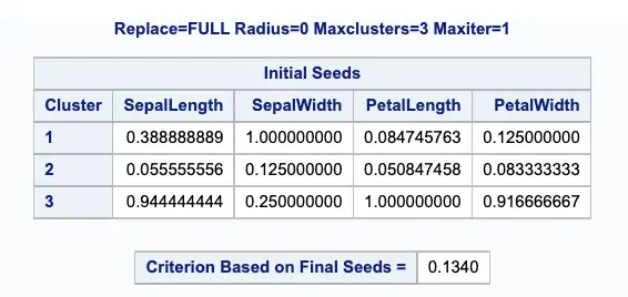
The below output displays the table of initial seeds used for each variable and cluster.
Next, PROC FASTCLUS produces a table of summary statistics for the clusters. The image below displays the number of observations in the cluster (frequency) and the root mean squared standard deviation.
The next two columns display the largest Euclidean distance from the cluster seed to any observation within the cluster and the number of the nearest cluster.
The last column of the table displays the distance between the centroid of the nearest cluster and the centroid of the current cluster.

It is useful to study further the clusters calculated by the FASTCLUS procedure. One method is to look at a
frequency tabulation of the clusters with other classification variables. The following statements invoke the
FREQ procedure to cross-tabulate the empirical clusters with the variable Species:
proc freq data=tree;
	tables cluster*species / nopercent norow nocol plot=none;
run;
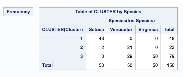
The output of the Proc FREQ procedure displays the marked division between clusters.
Visualizing Clusters
The optimal number of clusters from our example comes out 4. We need to check whether or not the clusters overlap with each other in terms of their location in the k-dimensional space of 4 variables.
It is not possible to visualize clusters in 4 dimensions. To work around this problem, we can use canonical discriminant analysis or any other data reduction technique that creates a smaller number of variables that are linear combinations of the four clustering variables.
The new variables, called canonical variables, are ordered in terms of the proportion of variance in the clustering variable that is accounted for by each canonical variable. So the first canonical variable will account for the largest proportion of the variance.
So, If you have more than two variables, you can use the CANDISC procedure to compute canonical variables
for plotting the clusters.
The goal of variable reduction is to find out which variables yield the largest difference among groups, and then those insignificant variables can be ignored in discriminant analysis.
We will be using the PROC PRINCOMP procedure for Variable reduction. The principal component analysis aims to reduce highly correlated variables into a small number of principal components.
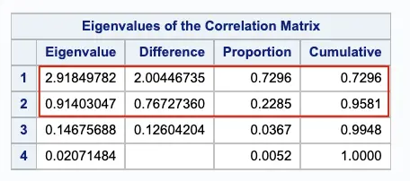
In this case, we retain the first two principal components.
Plotting the two canonical variables generated from PROC PRINCOMP, Prin1 and Prin2.
ods graphics / reset width=6.4in height=4.8in imagemap;

proc sgplot data=princomp;
	scatter x=prin1 y=prin2 / group=species;
	xaxis grid;
	yaxis grid;
run;

ods graphics / reset;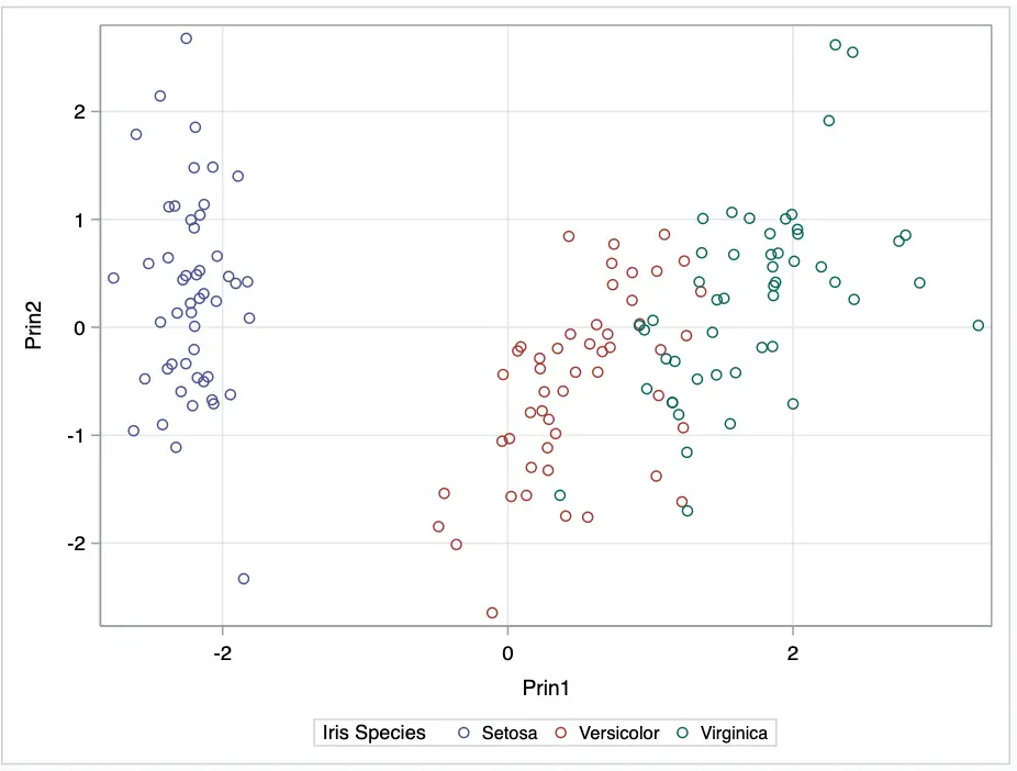
Using our analysis, we can see three clusters of different colours.
To summarize:
- PROC FASTCLUS procedure is suitable for large data sets.
- PRINCOMP performs a principal component analysis and outputs principal component scores.
- PROC SGPLOT is used to plot the analysis variables.

