Jupyter Notebook Tutorial: A Comprehensive Guide for Data Scientists

Don’t you just despise the frustration of sifting through data that seems more like an unsolvable knot than a clear path to insights? We get it, and we’re here to help.

Welcome to our Jupyter Notebook Tutorial, your lifeline in the choppy seas of data analysis. This guide is your key to unravelling the complexities of Jupyter Notebook, a game-changing tool that can transform the way you handle data.

We’ll start from the basics and walk you through the advanced features, turning this formidable tool into your trusted ally.

Jupyter Notebook Tutorial: A Comprehensive Guide for Data Scientists

Are you curious about why Jupyter Notebook is the talk of the town among data scientists? Wondering why it has become such an essential tool in the field?

Well, Jupyter Notebook, an open-source web application, allows you to create and share documents that contain live code, equations, visualizations, and narrative text.

The ability to write code, see the output, and provide explanations all in one place makes it a powerful tool for data analysis, statistical modelling, data visualization, and machine learning.

It supports over 40 programming languages, including Python, R, Julia, and Scala. The interactive nature of Jupyter Notebook makes it a perfect choice for data exploration and presenting data analysis results.

How to Install Jupyter Notebook?

Ready to get started with Jupyter Notebook? Let’s walk through the installation process together. Whether you’re on Windows, MacOS, or Linux, getting Jupyter Notebook up and running on your machine is a breeze.

For starters, you need to install Python. Jupyter Notebook is a Python library and requires Python to run. The easiest way to install Python and Jupyter Notebook is through the Anaconda distribution. Anaconda conveniently installs Python, the Jupyter Notebook, and other commonly used packages for scientific computing and data science.

Link to full installation instructions: Jupyter Notebook Installation Guide

The installation process is quite similar for both Windows and MacOS, and we’ll use the Anaconda distribution, which simplifies the installation process and provides additional tools that are helpful for data analysis.

Here are the steps:

1. Download Anaconda

The first step is to download the Anaconda distribution of Python. Anaconda is a free distribution of Python that comes bundled with many popular scientific libraries and is ideal for machine learning and data analysis. You can download Anaconda from the official website.

Choose the Python 3. x version, as it’s the most current. Make sure to select the installer that matches your operating system.

2. Install Anaconda

• For Windows users:
  • Run the installer.
  • Click “Next”, and then “I Agree” to agree to the license.
  • When asked to choose an install location, use the default location suggested by the installer.
  • On the next page, check the box that says “Add Anaconda to my PATH environment variable.” This will ensure that your computer can find Anaconda when you need to run it from the command line. Then, click “Install.”
• For MacOS users:
  • Open the installer you downloaded and you’ll see a window like this:

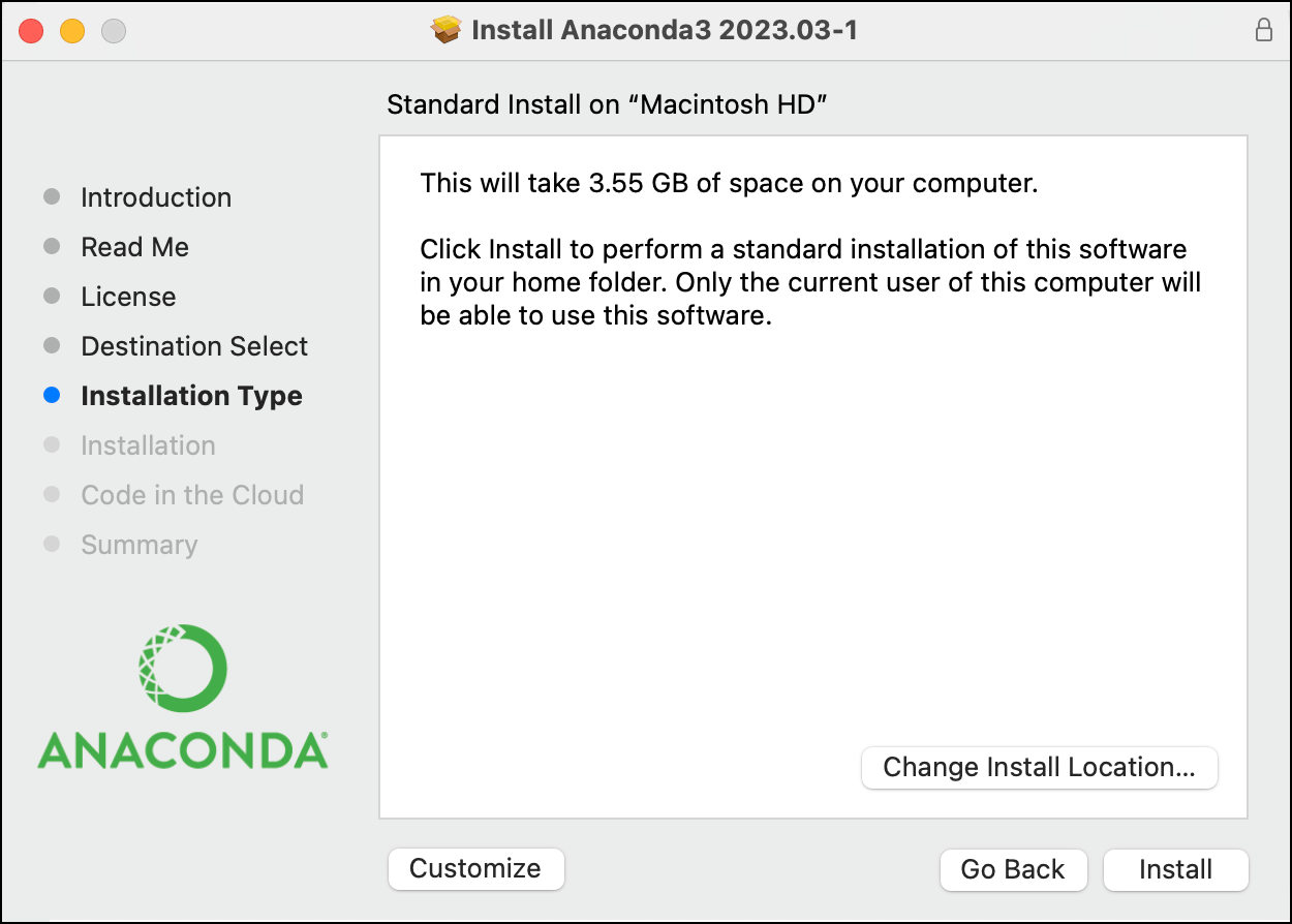
• Click on “Continue”, agree to the license, and then choose the install location. Use the default location suggested by the installer.
• Then, click on “Install”.

3. Verify the Installation

After the installation is complete, you can verify that it was successful by opening a command prompt (on Windows) or terminal (on MacOS) and typing the following command: jupyter notebook

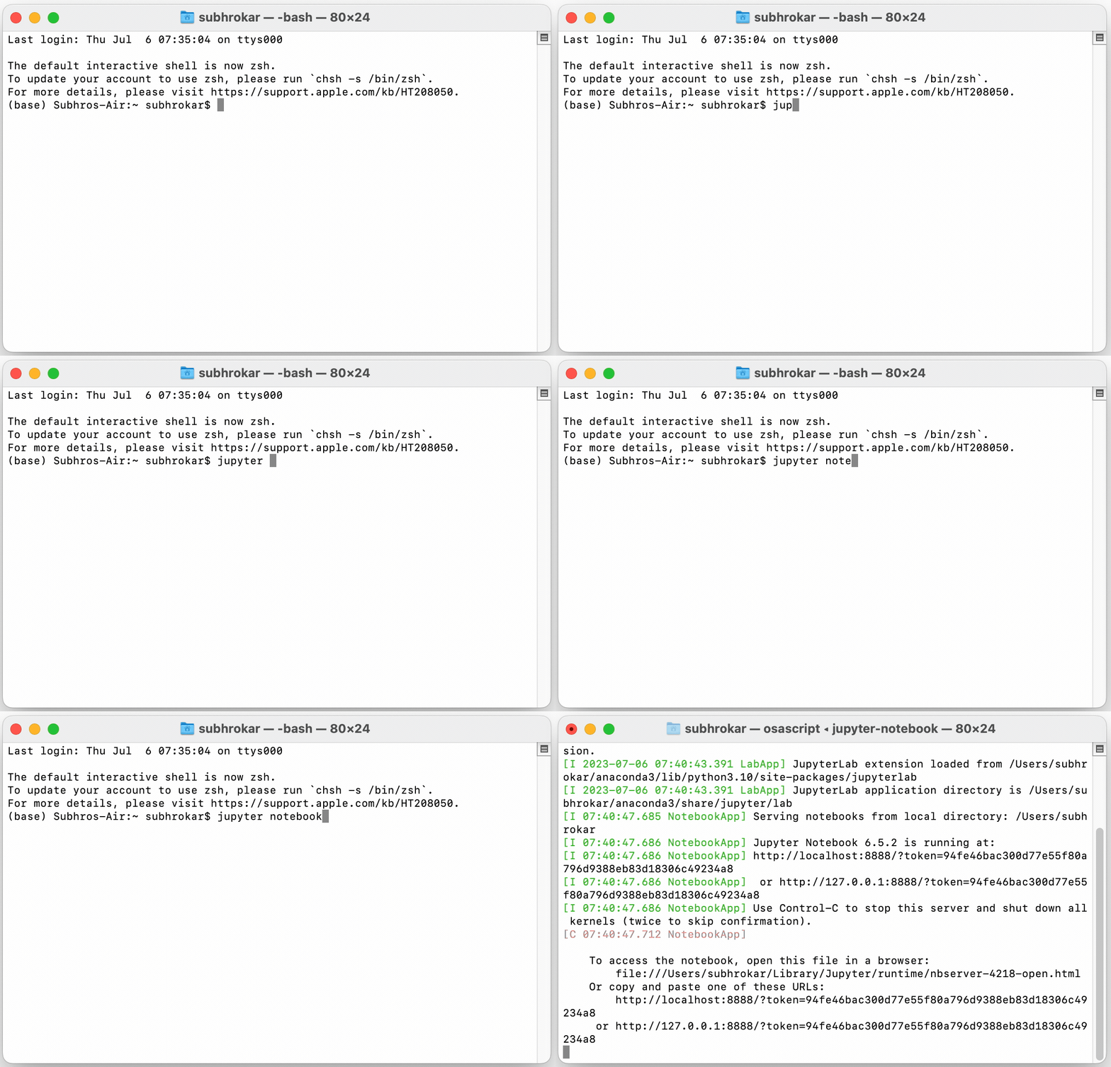
This should open a new tab in your default web browser with the Jupyter Notebook interface.

And that’s it! You have installed Jupyter Notebook using Anaconda.

How to open Jupyter Notebook?

Whenever you want to start Jupyter Notebook, you just need to open a command prompt or terminal and type: jupyter notebook

You are now ready to start using Jupyter Notebook for your data science projects!

What About Running Jupyter Notebook Online?

Did you know you can also use Jupyter Notebook on the cloud? You might be wondering, why to use the cloud when you can run Jupyter Notebook locally. Let’s unravel the benefits together.

Running Jupyter Notebook on the cloud comes with many perks. You can access your notebooks from anywhere, share them easily with colleagues, and take advantage of powerful cloud computing resources. This setup is particularly useful for working on large datasets and resource-intensive computations that your local machine may struggle with.

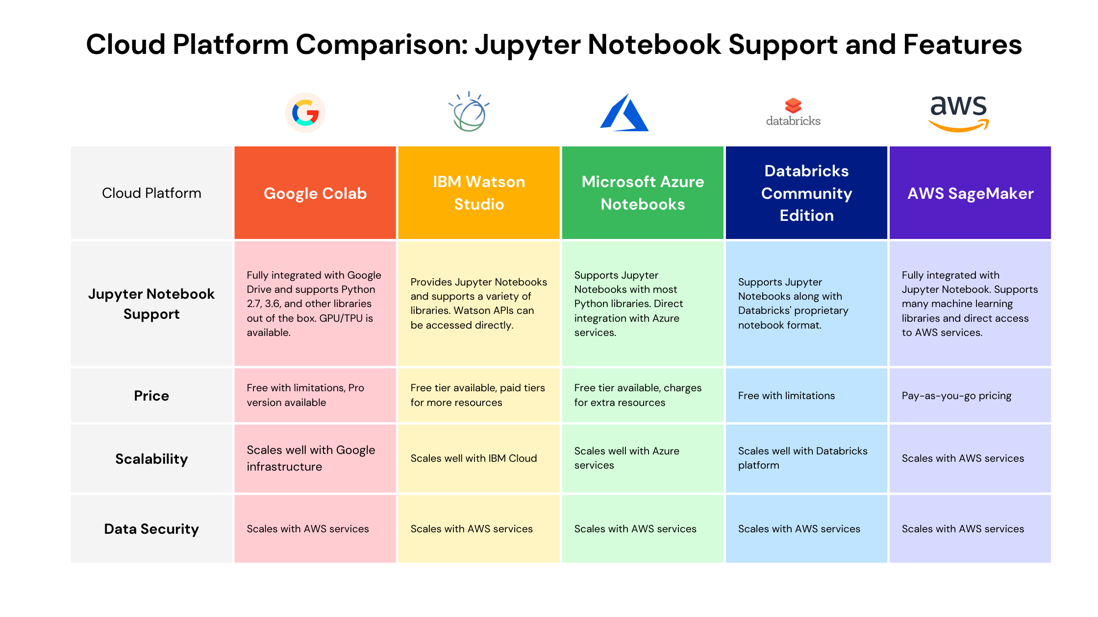
Many cloud platforms offer support for Jupyter Notebooks, including Google Colab, Microsoft Azure, and IBM Watson. Among these, Google Colab is a popular choice because it provides free access to GPU resources, making it a great platform for machine learning tasks.

Google Colab is a free cloud service that supports free GPU and is based on the Jupyter Notebooks environment. It’s perfect for machine learning, data analysis, and more. Google Colab notebooks are stored in Google Drive and can easily be shared with others. They provide an interactive learning environment and work seamlessly with other Google services.

Microsoft Azure Notebooks is another cloud-based Jupyter Notebook service similar to Google Colab. It offers free access with limited computational resources. It’s deeply integrated with Azure’s cloud storage, Azure Machine Learning, and other services provided by Microsoft.

IBM Watson also provides an interactive, collaborative, cloud-based environment where you can work with your data. Watson allows you to analyze data using Python and other languages, all in one place. It’s used extensively in businesses, particularly for predictive data analysis.

Databricks Community Edition is a free version of the Databricks platform that provides access to a micro-cluster as well as a cluster manager and notebook environment, allowing you to execute your code right from the cloud.

AWS SageMaker is a comprehensive service by Amazon that allows developers and data scientists to effortlessly build, train, and deploy machine learning models. It comes with fully managed Jupyter Notebook instances which serve as an efficient platform for writing code, visualizing data, and sharing results. Starting with creating a notebook instance, you can utilize the Jupyter dashboard to create new notebooks for machine learning experimentation, analyze data, and create models.

The Genesis of Analysis: Creating a Notebook in Jupyter

Once you’ve installed Jupyter Notebook and you’re ready to begin, the first step is creating a notebook. Let’s walk through the process:

1. Naming Your Notebook: Once you start Jupyter Notebook (typically by running the command jupyter notebook in your terminal or command prompt), your browser will open a new tab with Jupyter’s dashboard. Here, you can create a new notebook by clicking on ‘New’ and selecting ‘Python’ (or the kernel of your choice). The notebook will open in a new tab, named ‘Untitled’ by default. To rename, click on ‘Untitled’, type your preferred name, and hit ‘Rename’.

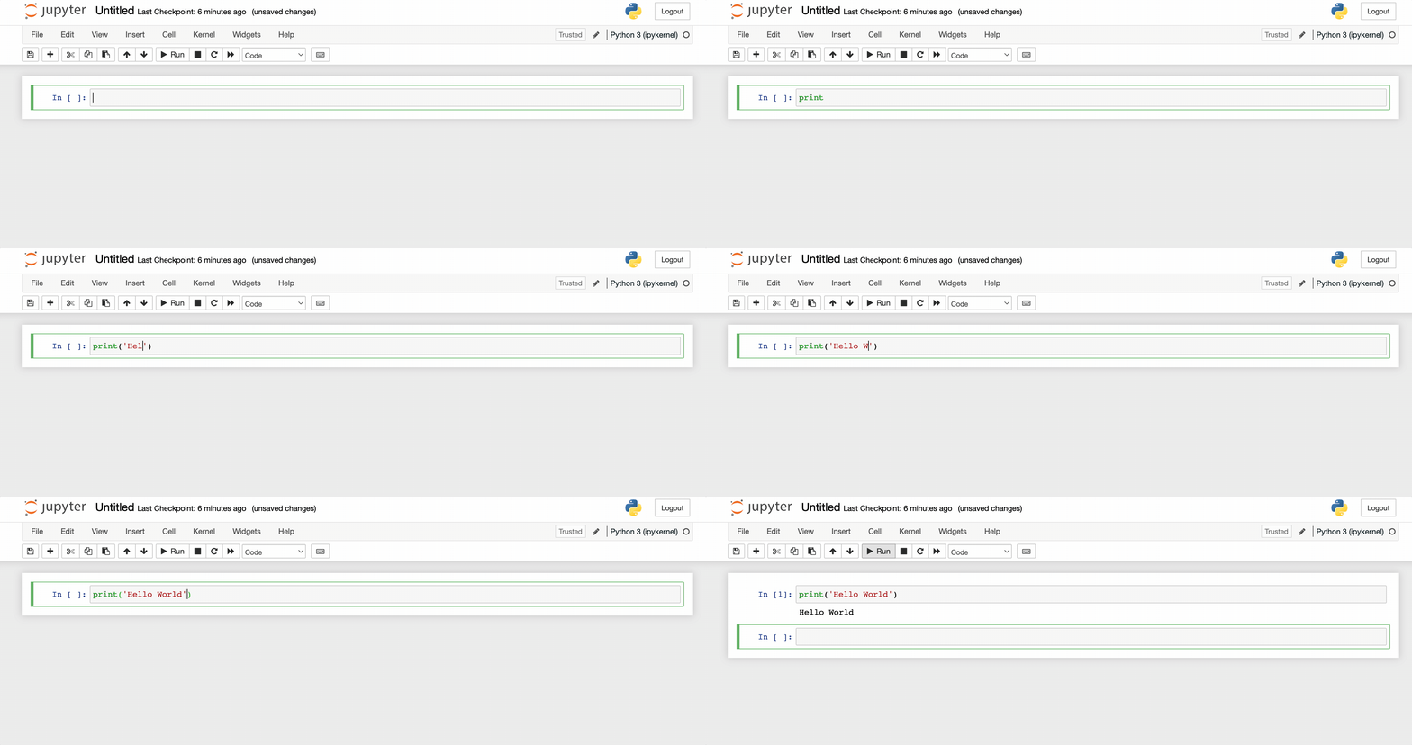
2. Running Cells: In your newly created notebook, you’ll see a single empty cell. You can type Python code directly into the cell and run it by clicking the ‘Run’ button on the toolbar or using the Shift + Enter keyboard shortcut. The results will appear directly below the cell.

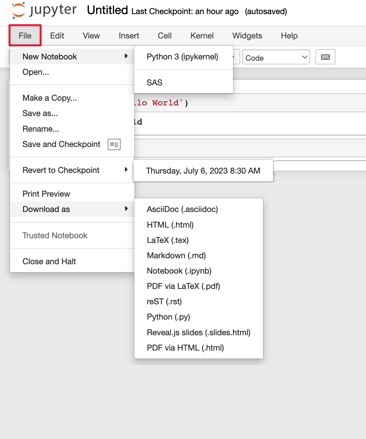
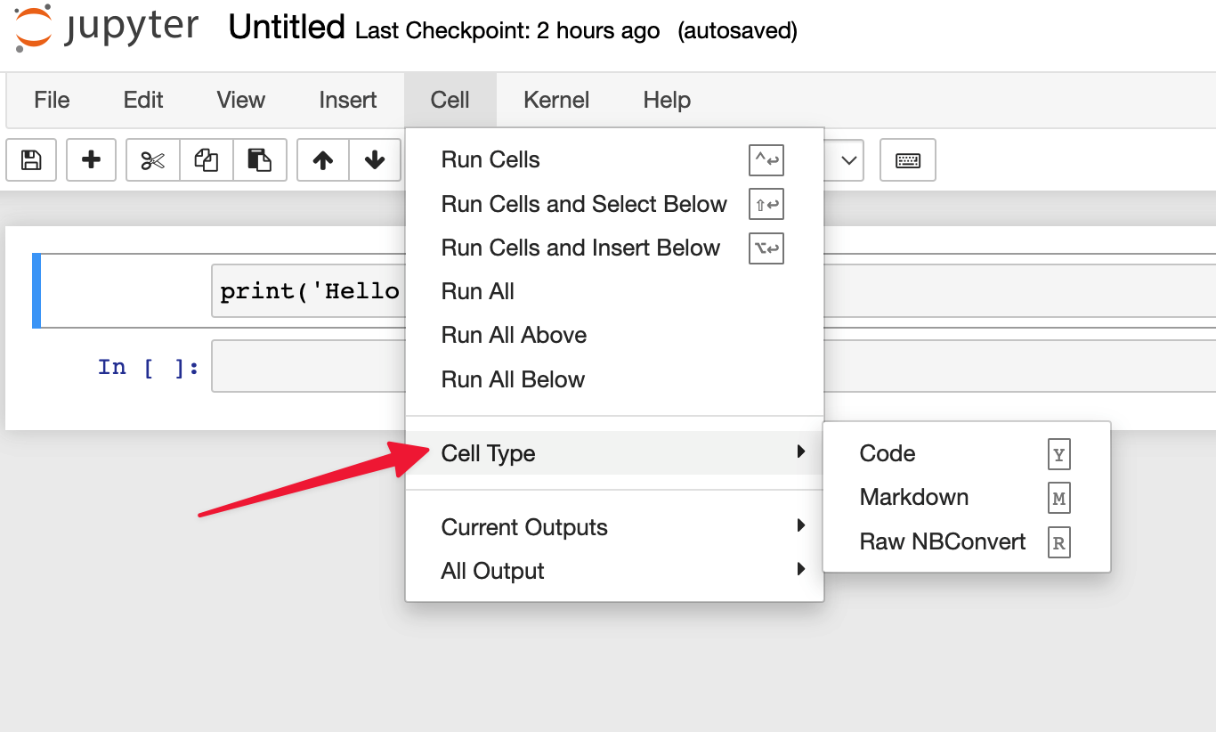
3. The Menus: The menu bar at the top of the notebook offer diverse options. ‘File’ lets you create new notebooks, open existing ones, save, rename, or download your current notebook. ‘Edit’ provides options for cutting, copying, and pasting cells. ‘View’ controls the visibility of the header and toolbar. ‘Insert’ allows you to insert new cells, and ‘Cell’ lets you run, stop, or change the type of cells.

4. Starting Terminals and Other Things: From the ‘New’ dropdown menu in the dashboard, you can also start a new terminal or text file or open a new folder.

5. Viewing What’s Running: You can view all running notebooks by clicking on the ‘Running’ tab in the dashboard. This shows all notebooks currently running on your system, along with an option to shut them down.

Creating and managing a Jupyter Notebook is intuitive and straightforward, thanks to its user-friendly interface. Now that you know how to create a notebook, name it, run cells, use the menu, and view running notebooks, you’re all set to start your data analysis journey with Jupyter!

Adding Color to Your Analysis: Incorporating Rich Content in Jupyter Notebooks

One of the reasons Jupyter Notebook has become a staple in the data science world is its ability to combine rich, formatted text with code in an easily navigable document. Let’s explore how you can incorporate rich content into your notebooks:

1. Cell Types: In Jupyter Notebook, there are primarily three cell types: code, markdown, and raw. ‘Code’ cells contain code to be executed by the kernel. ‘Markdown’ cells contain text formatted using Markdown and display their output in place when the Markdown cell is run. ‘Raw’ cells are not evaluated by the notebook.

2. Styling Your Text: Markdown cells support standard Markdown syntax for formatting text. You can create bold text with **bold text**, italic text with *italic text*, and strikethrough with ~~strikethrough~~.

3. Headers: Headers and sub headers can be created in Markdown cells using #. A main header can be created with a single #, sub headers with ##, and so on up to six levels deep.

4. Creating Lists: You can create ordered and unordered lists in Markdown. Unordered lists can be created using *, -, or + before each item. Ordered lists can be created by numbering each item, like 1. Item.

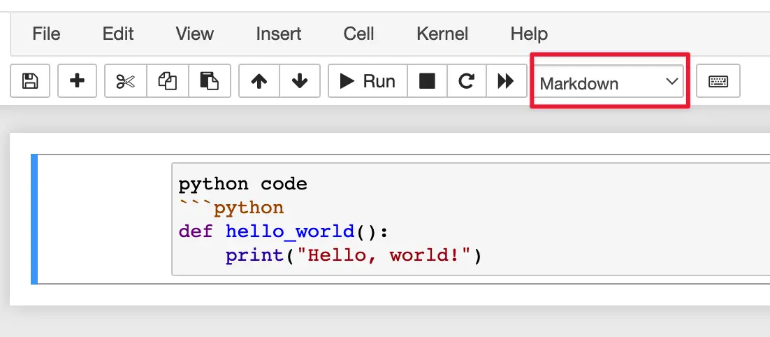
5. Code and Syntax Highlighting: When you write code in a ‘Code’ cell, Jupyter Notebook automatically highlights the syntax according to the programming language. You can also include code with syntax highlighting in a Markdown cell by enclosing the code within triple backticks (“`) and specifying the programming language.

Here’s an example for Python:

For a more in-depth exploration of using markdown in Jupyter Notebook, I recommend checking out this comprehensive guide on Medium. It’s a fantastic resource that dives deep into the nuances of markdown within Jupyter.

Decoding the Language of Jupyter: Understanding Jupyter Notebook Commands

Once you’re up and running with Jupyter Notebook, mastering the commands is your next big step. These commands, or shortcuts, can make your experience with Jupyter Notebook smoother and more efficient.

Keep in mind that these shortcuts are geared towards Windows and Linux users. For those using a Mac, the keys for Ctrl, Shift, and Alt are a bit different:

• Ctrl is the command key (⌘)
• Shift remains as Shift (⌧)
• Alt is the option key (⌥)

It’s essential to understand that the Jupyter Notebook App operates in two distinct modes: command mode and edit mode. Here are some shortcuts that work in both modes:

• Shift + Enter: Executes the current cell and then selects the cell below.
• Ctrl + Enter: Executes the selected cells.
• Alt + Enter: Executes the current cell and then inserts a new cell below.
• Ctrl + S: Saves and creates a checkpoint.

So, let’s unravel some of the most essential Jupyter Notebook commands:

1. Command Mode and Edit Mode: Understanding these two modes is crucial. When you select a cell, you’re in Command Mode (the cell border is blue), and you can perform notebook-level actions. Press Enter to switch to Edit Mode (cell border is green), where you can modify the cell’s content.
2. Running a Cell: To run a cell and see the output, you can use Shift + Enter. This also moves you to the next cell. If you prefer to stay on the same cell, use Ctrl + Enter.
3. Creating New Cells: In Command Mode, A inserts a new cell above the current cell, while B inserts a new cell below.
4. Copy, Cut, and Paste Cells: Still, in Command Mode, you can use C to copy a cell, X to cut it, and V to paste it below the current cell.
5. Deleting Cells: Pressing D twice in Command Mode will delete the current cell.
6. Changing Cell Types: In Command Mode, press Y to change a cell to a code cell, M to change it to a markdown cell.
7. Saving the Notebook: To save your work, you can press S in Command Mode.
8. Stopping Cell Execution: If your code is stuck in a loop or taking too long to execute, you can stop it by pressing I twice in Command Mode.
9. Restarting the Kernel: If you need to restart your notebook due to some technical issues, you can use 0 twice in Command Mode.

These are just a few commands to get you started. As you continue your journey with Jupyter Notebook, you’ll come across many more commands that will make your data analysis faster and more efficient. Practice them, and soon enough, they’ll become second nature to you!

So, are you ready to speak Jupyter’s language?

As a developer, I like to use shortcuts and snippets as much as I can. They just make writing code a lot easier and faster. Here’s a rundown of the most commonly used commands and their descriptions:

1. Command Mode Shortcuts (press Esc to enable)

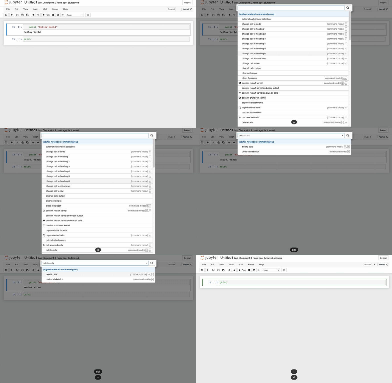
• Enter: Enter edit mode
• H: Show all shortcuts
• Up / K: Select the cell above
• Down / J: Select the cell below
• A / B: Insert cell above/below
• X: Cut selected cells
• C: Copy selected cells
• V: Paste cells below
• Z: Undo cell deletion
• Y: Change cell type to Code
• M: Change cell type to Markdown
• S: Save and checkpoint
• P open the command palette.
  This dialog helps you run any command by name. It’s useful if you don’t know some shortcut or when you don’t have a shortcut for the wanted command.

2. Edit Mode Shortcuts (press Enter to enable)

• Esc: Switch to command mode
• Ctrl + Enter: Run cell
• Shift + Enter: Run cell, select below
• Alt + Enter: Run cell, insert below
• Ctrl + S: Save and checkpoint
• Ctrl + Z: Undo
• Ctrl + Shift + Z: Redo
• Tab: Code completion or indent
• Shift + Tab: Tooltip

3. Menu Commands

• File -> Download as: Download your notebook in different formats like HTML, PDF, .ipynb, etc.
• Kernel -> Restart: Restart the kernel (ends the kernel session).
• Kernel -> Restart & Clear Output: Same as above but also clears output from all cells.
• Kernel -> Restart & Run All: Same as above but runs all cells in order.

4. Magic Commands

• %run: Run a Python script as a program.
• %load: Insert the code from an external script.
• %who: List all variables of global scope.
• %reset: Delete all variables/names defined in the interactive namespace.
• %history: Show command input history.
• %matplotlib inline: Render Matplotlib plots inline within the notebook.

We’ve prepared a handy Jupyter Notebook Shortcuts Cheatsheet for you.

How to Use Jupyter Notebook for Python

Curious about how Python and Jupyter Notebook work together? You’ve come to the right place! Python is one of the most widely used programming languages in the world, and when it’s combined with Jupyter Notebook, it becomes a data scientist’s best friend.

In Jupyter Notebook, Python code is written in cells, which are blocks that can individually hold code, visuals, or text. These cells can be executed independently or collectively, and they immediately display output beneath them when run. This makes for an interactive and iterative coding experience.

Let’s go through a simple Python example in Jupyter Notebook.

1. Creating a Notebook: To start with, open Jupyter Notebook and create a new Python notebook. You can do this by clicking on the “New” button and selecting “Python” from the dropdown. Image suggestion: Screenshot of creating a new Python notebook in Jupyter.
2. Writing Code: In the empty cell, write a simple Python command, such as print('Hello, World!'). Image suggestion: Screenshot of writing the Python command in a cell.
3. Executing Code: To execute the code, simply press Shift + Enter. You’ll see the output (‘Hello, World!’) appear right below the cell. Image suggestion: Screenshot of executing the cell and the output.
4. Adding More Cells: To add more cells, click on the “+” button on the toolbar. This way, you can write and execute multiple lines of code independently.

Python’s extensive libraries, such as NumPy for numerical operations, pandas for data manipulation, Matplotlib for plotting, and sci-kit-learn for machine learning, can also be used in the Jupyter Notebook. They can be imported as usual at the start of the notebook with commands such as import numpy as np.

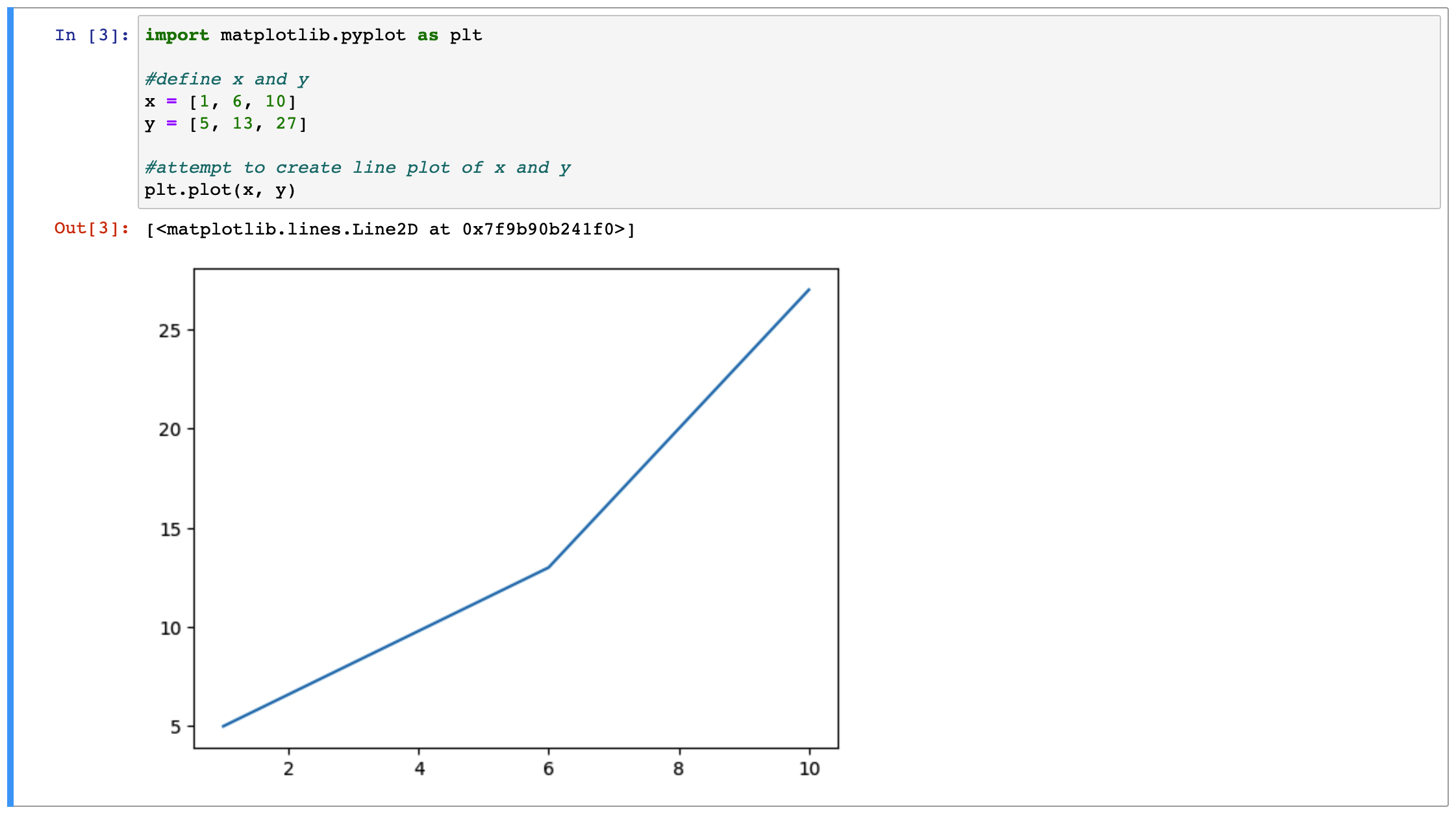
One key feature of using Python in Jupyter Notebook is the ability to display plots and graphs inline, which means the visualizations appear right within the notebook. This is done by using the magic command %matplotlib inline before any plotting commands.

So, are you ready to leverage the power of Python in Jupyter Notebook and revolutionize your data analysis process?

Further learning: Python for Data Analysis: A Tutorial for Beginners

Expanding Your Jupyter Experience: A Look at Jupyter Notebook Extensions

Extensions in Jupyter Notebook are like the extra features in a car – they enhance your experience, making the journey more comfortable and efficient. These extensions provide additional functionality that isn’t included in the default Jupyter Notebook package. Let’s explore some of the most useful Jupyter Notebook extensions:

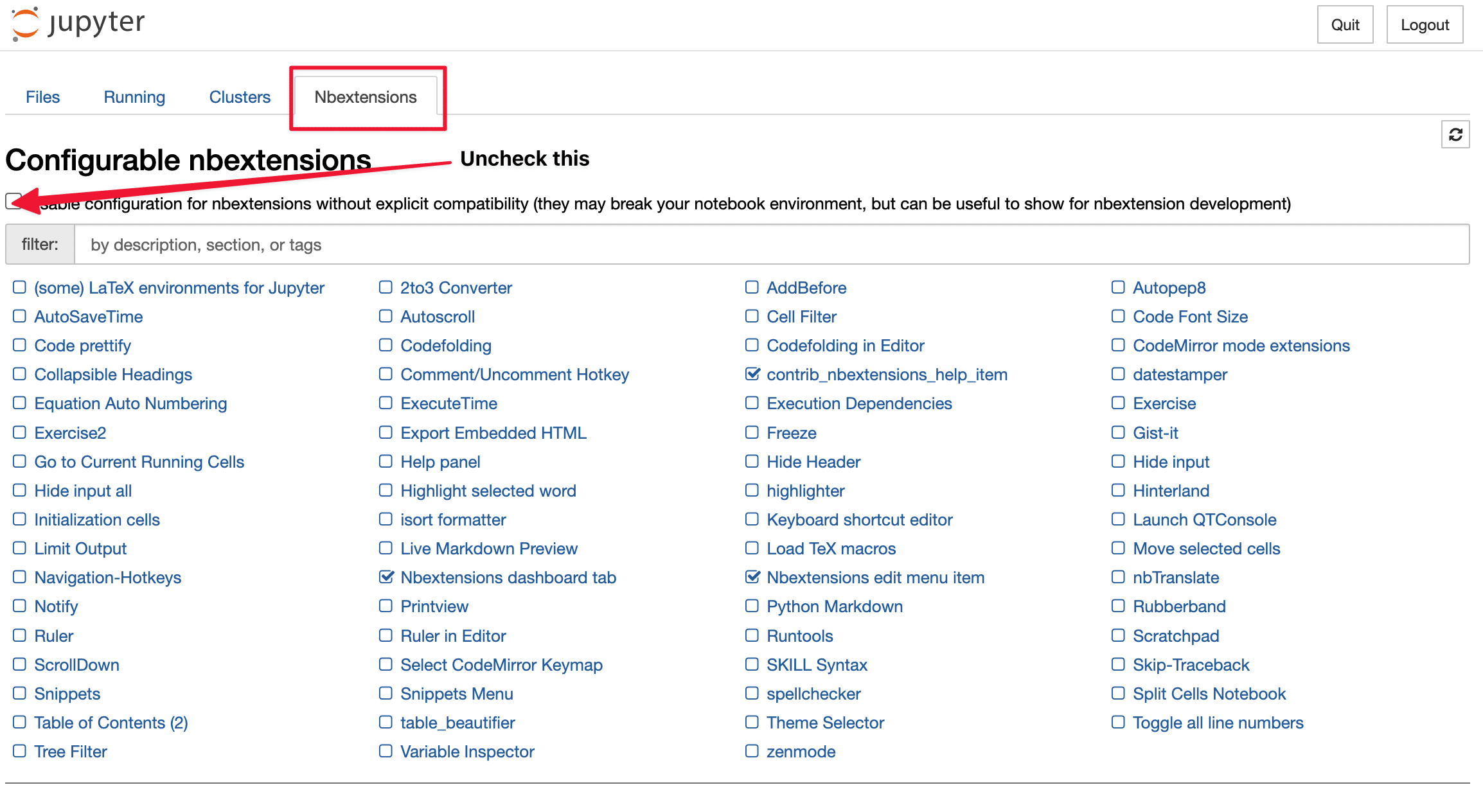
1. Nbextensions: This is actually a collection of extensions that add functionalities like spell-check, code folding, and execution time indicators. You’ll need to install the jupyter_contrib_nbextensions package and enable the Nbextensions tab to access these features.

1. JupyterLab: JupyterLab is the next-generation interface for Jupyter Notebook, offering a more integrated and user-friendly environment. It allows multiple notebooks to be opened side by side and supports file exploration, text editing, and markdown rendering.
2. RISE: An acronym for “Reveal.js – Jupyter/IPython Slideshow Extension,” RISE enables you to turn your Jupyter Notebooks into interactive slideshows. This is perfect for presentations where you need to show both your code and your results.
3. Jupyter Widgets: Also known as ipywidgets, these interactive HTML widgets can make your notebooks more interactive. They’re useful for data exploration, data visualization, and building GUIs within your notebooks.
4. Voila: Voila transforms Jupyter Notebooks into standalone web applications. It allows users to execute existing cells but not modify the code, which makes it great for sharing results without exposing your code.

To install these extensions, you typically use pip or Conda (depending on your Python environment), and then enable them in Jupyter Notebook. Remember, extensions can significantly enhance your Jupyter Notebook experience, but they also require resources, so be mindful of which and how many you install.

Link to full installation instructions: Installing jupyter_contrib_nbextensions

So, are you ready to supercharge your Jupyter Notebook experience with these extensions?

Note: Some of these extensions may not work with all versions of Jupyter Notebook. Please check the compatibility before installation.

Sharing Your Insights: Exporting Notebooks in Jupyter

After hours of data wrangling and analysis in your Jupyter Notebook, you’ve gained valuable insights, and now it’s time to share them. One of Jupyter’s advantages is its ability to export notebooks in various formats using a tool called nbconvert. Here’s how you can do it:

1. What is nbconvert?:nbconvert is a tool built into Jupyter that converts your notebook (.ipynb file) into another format such as HTML, PDF, LaTeX, Markdown, reStructuredText, or even a Python script.

2. Example Usage: To use nbconvert, you’ll need to open your terminal or command prompt and navigate to the directory containing your notebook. Here’s an example of how to convert a notebook to an HTML file:

jupyter nbconvert --to html --template basic mynotebook.ipynb

Replace ‘YourNotebook.ipynb’ with the name of your notebook. After running this command, you’ll have an HTML version of your notebook in the same directory.

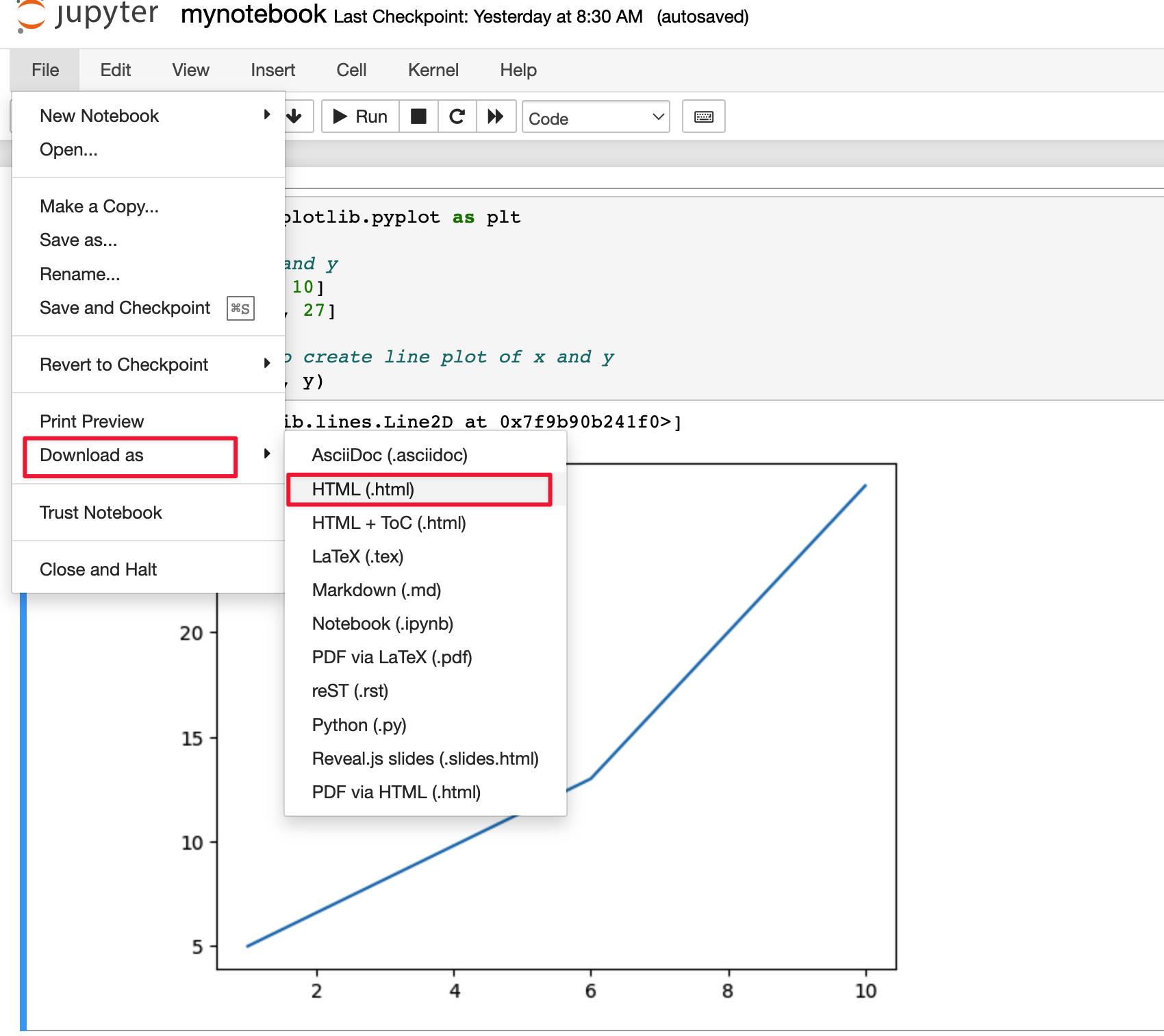
3. Use the Menu: If you prefer not to use the command line, you can also export your notebook using Jupyter’s menu. With your notebook open, go to the ‘File’ menu, then ‘Download as’. You’ll see a list of formats you can export your notebook to. Simply click on the desired format, and your browser will download the converted file.

Exporting your Jupyter Notebook allows you to share your results and insights more effectively with others, especially those who don’t use Jupyter Notebook. Whether they prefer to view your work in a web browser (HTML), as a document (PDF or LaTeX), or in a markdown viewer, Jupyter Notebook has gotten you covered.

Wrapping Up Our Journey Through Jupyter Notebook

Congratulations on completing our Jupyter Notebook tutorial! We’ve covered everything from installation and commands to leveraging cloud-based solutions and mastering Python in an interactive environment.

Jupyter Notebook’s powerful combination of code execution, rich text, mathematical expressions, and visualizations makes it a go-to tool for data scientists worldwide.

Keep exploring and coding to create stunning data projects. You’re well on your way to becoming a proficient data scientist with Jupyter Notebook as your dynamic tool.

Leave your questions in the comments below, and we’ll do our best to help. Every line of code is a step forward in your data science journey!